Hi,
As an Excel user, sometimes we store or transfer an Excel file, which contains some confidential data. It becomes a basic need to protect it either in a way that the user either can only see the data (read-only) or can modify it also. Microsoft Excel gives us few protection features, which are strong enough to protect your confidential data from most of the suspicious elements. But always keep in mind that Excel is not a vault, where you can store and protect your data, as protection features are not that great as they supposed to be because the purpose of Excel is just to analyze the data.
In this post, we will understand the following levels of protection-
1- Complete workbook protection
2- Worksheet level protection
3- Protect selected range
4- Protect workbook Structure and window
5- Assign the different password to different ranges in one worksheet
1.Complete Workbook Protection-
This protection level will set a password on the workbook. The moment a user tries to open, it will ask for the password.
Isn’t it cool?
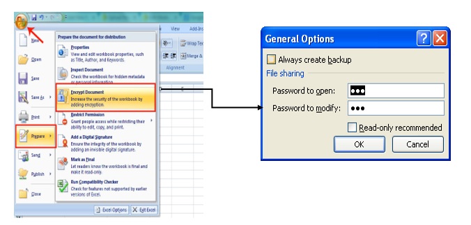
Ms-Office 2007 User-
1- Click on Office Button
2- Prepare
3- Encrypt document
4- Apply password & Confirm password
5- Ok
6- Save the document
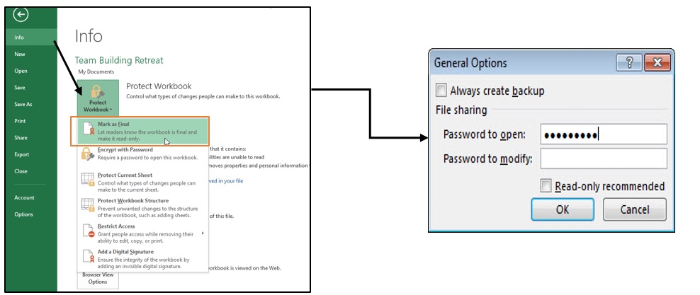
Ms-Office Version 2010 and above-
- File
- Info
- Protect workbook
- Encrypt with password
- Apply Password
- Ok
- Save y0ur file
Note: To remove the password just follow the same steps as explained above. Remove the password and save the file.
2.Worksheet level protection –
This will help us in protecting the desired worksheet out of the complete workbook.
Steps to protect worksheet-
- Go to Review tab
- Protect sheet
- Apply Password
- Re-Enter password
- Ok
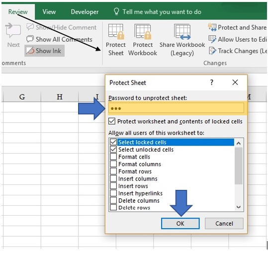
You can give following permission to the users during the password protection-
- A- Select Locked Cells- On the protection tab of the format cells dialogue box is checked would be locked. By default users allowed to select locked cells.
- B- Select Unlocked cells- If unchecked this option password would not be applied because this option is interconnected with locked cells.
- C- Format Cells- By checking this option, we are giving permission to users that can change the formatting of cells after the password protection.
- D- Format columns- By enabling this option, we can change the columns width and hide the columns.
- E- Format Rows- BY checking this option, we can change the rows height and can hide them.
- F- Insert columns- we can insert columns after the protection.
- G- Insert rows- we can insert rows after the protection.
- H- Insert hyperlinks- we can insert, edit the hyperlink.
- I- Delete columns- we can delete the columns as well.
- J- Delete rows- we can delete the rows as well
- K- Sort- Checking this confirms the availability of Sort on the protected worksheet
- L- Use AutoFilter- Checking this confirms the availability of Filter on the protected worksheet
- M- Use PivotTable reports- If we have already created a pivot table and enable this option while applying the password. You can edit.
- N- Edit objects – Make changes to graphical objects including maps, embedded charts, shapes, text boxes, and controls that we unlocked before we protected the worksheet. For example, if a worksheet has a button that runs a macro, we can click the button to run the macro
3. Protect selected range-
This will help us to protect a part of a sheet
Steps to protect a range-
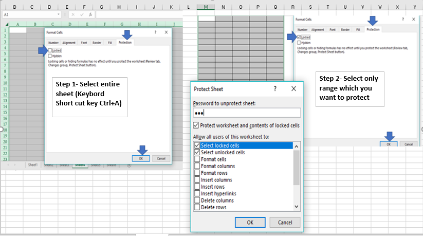
- Select the entire sheet by clicking on the top left corner of the sheet or press Ctrl+A
- Right-click -> format cells -> Go to protection tab -> uncheck “Locked”. (Note: to open number format you can also use shortcut key Ctrl+1)
- Select the desired cell or range then press ctrl+1 (Format cells)
- Go to protection tab then Checkmark on Locked
- Ok
- Review tab
- Apply Password and confirm password
- Ok
4. Protect workbook Structure and window–
Do you know, just protecting a worksheet is not enough? A protected worksheet can be renamed or even can be deleted by the user. The user can also insert a worksheet. Here the need for workbook structure protection comes into the picture. This will ensure any worksheet of the workbook from deletion or insertion.
Steps to protect the workbook structure-
- Go to review tab
- Protect Workbook
- Make sure that there should be the check mark on the option Structure (Note: by default, it comes with the check mark)
- Apply Password
- Ok
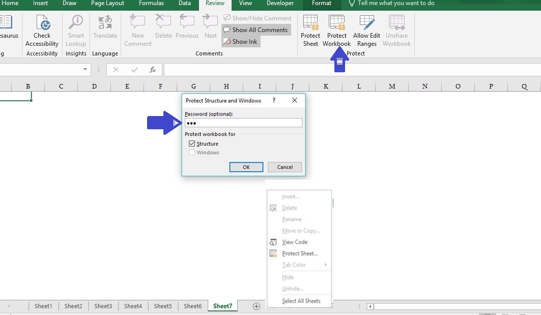
After the protection, no one can delete, edit or insert a new sheet.
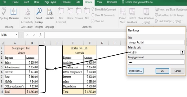
5. Assign the different password to different ranges in one worksheet –
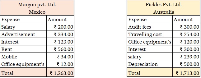
If we have two table on a worksheet and we want to protect each table with different passwords along with full worksheet protection with another password.
Steps for Assigning the different password to different ranges in one worksheet –
- Go to review tab
- Click “allow the user to edit range”
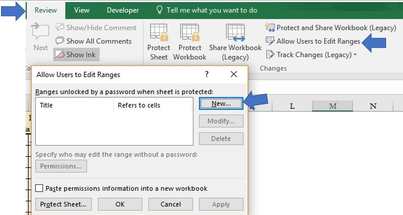
- Click on the New tab
- Give Title name
- Provide the Range
- Password and re-enter password
- Ok
Again, click on “New” then provide the different password for another table. Follow the same steps.
Once we provide different passwords to each table now click on Protect sheet and provide the different password to protect the sheet (see point 2 – Worksheet level protection (Protect Objects))
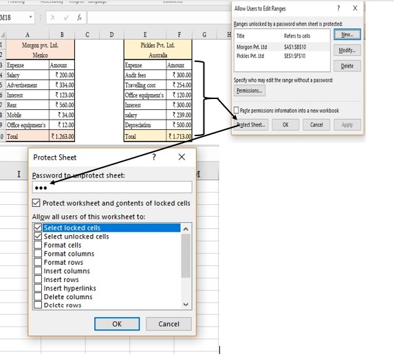
To unlock the protected ranges, follow the same process and enter the password.

If you like this post, then don’t forget to subscribe our channel and if any query post in comment box.
Stay connected and Happy Learning 😊