
Custom Number Formatting
Custom Number Formatting-
Sometimes when you download or import any data into Excel, its formatting looks weird. Dates get converted to numbers or Numbers are showing in scientific characters (2.34568E+12), Decimal points, Currency symbols, convert number into percentage, friction, Text format etc. For these unexpected formats we have a listed options available in under “Number format” feature, however apart from these formatting glitches, if we need only Days out of a date, 5 digits invoice number starting with “0” zeros, Numbers with certain decimal places etc., this feature can be used.
This post is all about data formatting in Excel. I hope you all are excited as I am. let’s get dive into the ocean of Excel Formatting.
- Date Format–
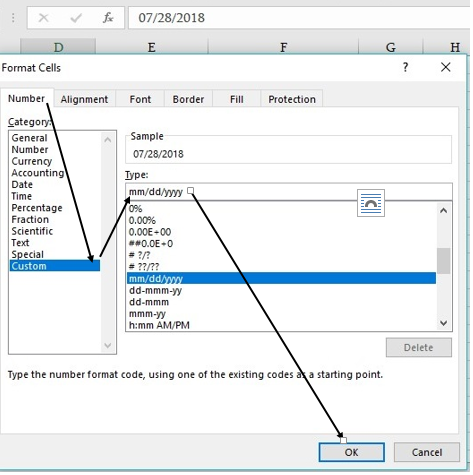
First, let’s through some light on date formats, as we can see in above screenshot, Sometimes when we type a date in a format like “07-28-2018”, it converts the format automatically into “7-28-18”,this is known as a single digit date format. To get rid of this auto formatting, follow the steps given below-
- Select the data contains all the dates.
- Right click and select Format cells(Ctrl + 1)
- Number tab -> custom
- Change the date format to – DD-MM-YYY
- Ok
Note: Although Excel always takes the date format of the computer. We can check the data format by pressing short cut key ctrl+; (Control+Semicolon) in any blank cell.
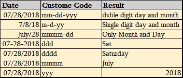
How custom format reacts on different combination-
- Typing “D” will show only day. Example “9”
- Typing “DD” will show day in two digits. Example “09”
- Typing “DDD” will show day in words (short form). Example “MON”
- Typing “DDDD” will show day in words. Example “Monday”
Similarly, to convert months/years, follow the same steps, instead of using “D” you will use “M”.
- Number Format-
2.1 Adding zero before number-
As we type any number that starts with Zero “0”, excel automatically omit zeros the moment one press enter. To prefix zeros, starting it with an apostrophe (‘) will solve the purpose but it will also convert a numerical data into text.
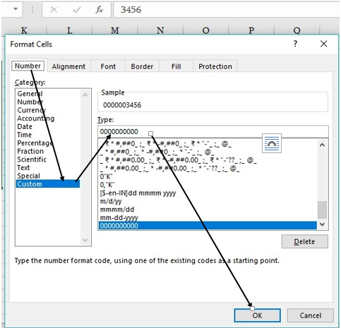
Prefixing zeros are much more reliable and easier using “Number Format”. Let’s take an example, out of a list of 10,000 invoice numbers containing some invoice numbers are of 4, 5 or 6 digits and the need is to keep a symmetry of 10 characters. Try the steps below –
- Select all the invoice numbers
- Open format cells (Ctrl+1)
- Number format -> Custom
- Enter ten Zeros (0000000000)
- Ok
2.2 Prefix thorough custom number formatting-
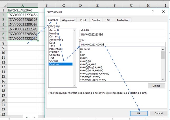
An invoice Number like this- INV#00022212345, which has text pre fixed and followed by numbers is standard in an organization. As per the need to keep all the invoice numbers symmetrical, prefixing of certain characters are required. Following process can help in the same:
- Select all the invoice numbers
- Right click and click on Format cell (Ctrl+1)
- Number Format -> Custom
- Remove General-
Note: The part of the invoice number that needs to be common must be entered in double inverted commas and insert zeros as per the requirement.
- “INV#000222” 00000
- Ok
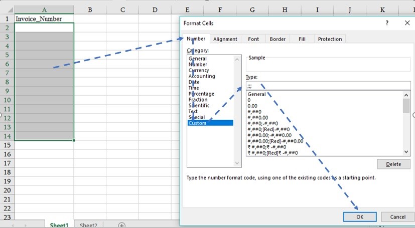
- Hide Cell contents-
Occasionally, if one need to hide the content of the cells following steps can be performed.
- Select your data range
- Right click and click on format cells (Ctrl+1)
- Number -> custom
- Remove General and type three times semicolon (;;;)
- Ok
Note: Three times semicolon will hide all the text and number. Two times or single time semicolon will hide only Numerical value.
- Convert Scientific number to Number format-
In Excel, any number that goes above 11 digits automatically converts into scientific numbers eg- (2.34568E+12). To get rid of this, one can use “Number format” by following below steps-
- Select range
- Right click and select format cells(Ctrl + 1)
- Go to custom and type hash # one time only
- Ok
Note: Even using hash # we can convert a number upto 15 digits, beyond it you must convert your number into text format or start with apostrophe (‘) symbol.
- Change font colour with custom number format-
Changing font colour of values in Excel can be done with the help of Custom Number format. There are 8 colours which custom format supports.
[Red] [Green] [Blue] [Yellow] [White] [Magenta] [Cyan] [Black]
- Select range
- Right click and select format cell (Ctrl+1)
- Custom number format
#, ##.00- Positive number format
(#, ##,00)- Negative number format
“-“- Zero value
“Text” @- Text format
| Value | Code | Remarks |
| 12.00 | [Green]#,###.00 | Format for positive number with two decimal places |
| -(34.00) | [Red](#,###.00) | Format for Negative number with two decimal places |
| – | “-“ | Format for highlighted Zero (Display dashes instead Zero) |
| Nurture Tech Academy | [Magenta]@ | Format for highlighted text |
- Repeat Characters with custom number –
To repeat the specific characters in your selected cells so that it will fill the column width with the same character, use Asterisk (*) symbol before the character.
| Values | Code |
| a********************* | @** |
| 1============= | #*= |
| *********************1 | **0 |
| 00000000000022 | *00 |
| 2,222*************** | #,###** |
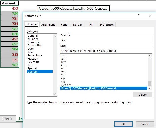
- Conditional based colour into custom number format-
We can highlight numerical data with conditions. For example, if we have a numerical value in which we want to highlight in Green colour those which are more than five hundred (>500) and Red colour for less than five hundred (<500).
- Select the range
- Right click and select format cell(Ctrl + 1)
- Custom number formatting
- Remove general and type this formula- [Green][>500];[Blue][<=500]
- Ok
If you have any query feel free to write down in the comment box or visit our website www.nurturetechacademy.in
Stay connected and Happy Learning 😊
360 total views, 3 views today
Tag:corporate training companies, corporate training companies in Delhi, corporate training courses, corporate training in delhi, corporate training programs, custom number formatting in excel, custom number formatting in microsoft Excel, custom number formatting in MS Excel, excel course online, excel courses online, excel online course, excel online training, excel training in delhi, excel training online, How can we use custom number formatting in Excel, How can we use custom number formatting in microsoft Excel, How to use custom number formatting in microsoft Excel, learn microsoft excel, learn ms excel online, learning excel online, learning microsoft excel, microsoft excel course, microsoft excel online training, microsoft excel training, ms excel learning, MS excel online training, ms excel training in delhi, online corporate training, online excel course, online excel training, online excel training courses

You may also like

Heat Map Chart through Radio Button in Excel
27 December, 2018
How to Create a Histogram Chart in Excel
22 November, 2018
Count Functions in MS Excel
12 November, 2018