How to use VLOOKUP with multiple tables

Hi,

As an excel user, when we are maintaining data on different tables or on different sheets however we want to pull the information on a single sheet from the tables. If we do type manually or copy and paste it, it will consume more time basically Its time taken process.

Let’s understand the problems first then we will discuss the solution in detail-

The Problem-

Below is an example with a dummy data-

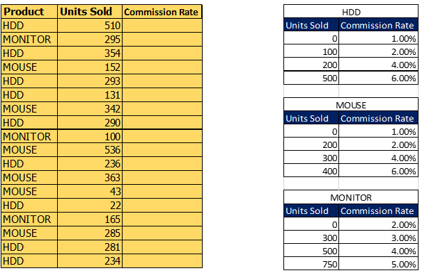
There are three tables with different Commission rate e.g. Table HDD, Table MOUSE, Table Monitor.

We want to get commission rate according to their Unit Sold given in second column of Excel sheet.

Step-1

In the example shown, there are three tables, so we have to define a Name with the help of Naming range option to each table.

How to define Naming range on table?

Select the Table->Go to Formulas tab-> Define Name-> Define Name in Name Box-> Ok

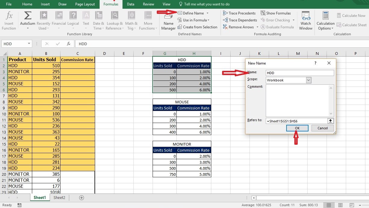
Repeat the process for another table and define Name i.e. Mouse, Monitor

Note: It would be good, give Name that should be like your product name so that it’s easy to find the value.

Step-2

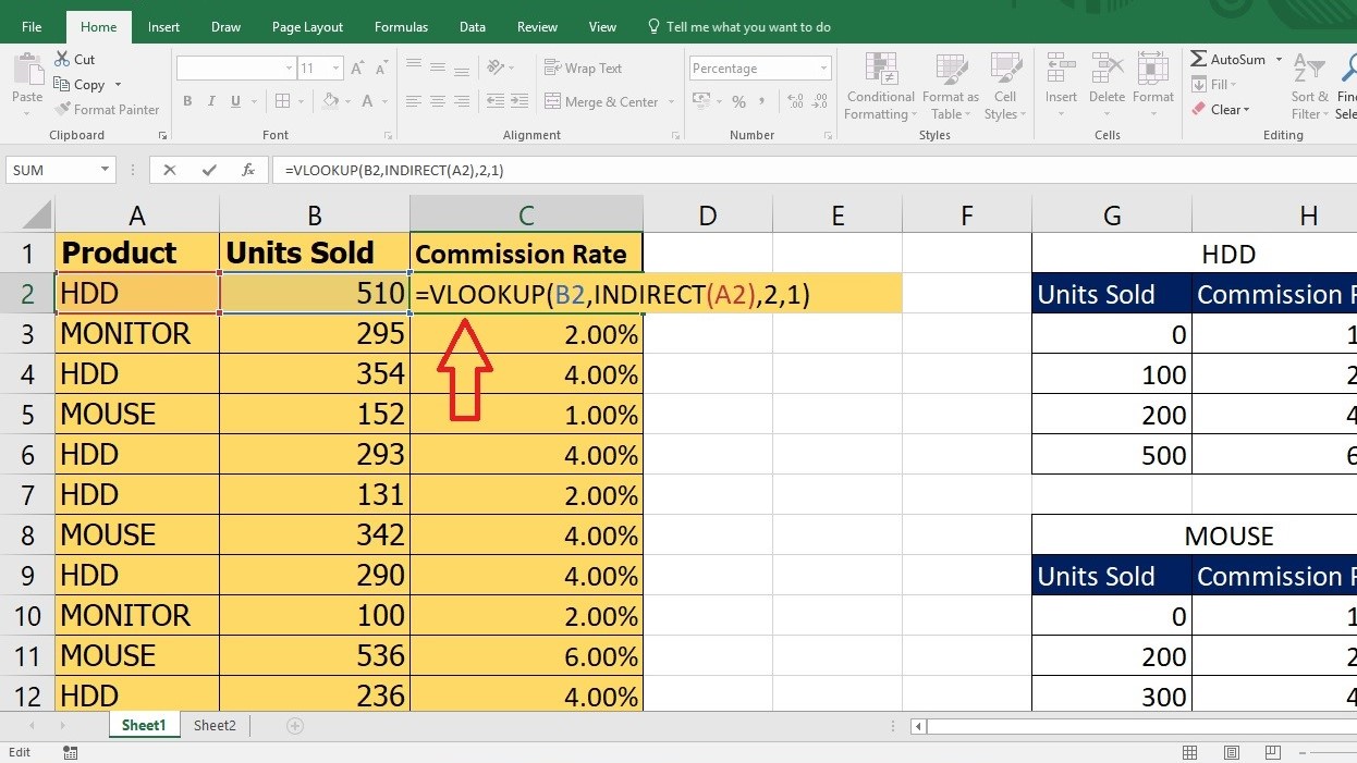
At the core, this is a standard VLOOKUP formula. The only difference is the use of INDIRECT to return a valid table array. INDIRECT function picks up the text in A2 (“HDD”) and resolves it the named range HDD, which resolves to G2:H6, which is returned to VLOOKUP.

Open your worksheet->type formula in column C2 i.e. “=VLOOKUP (B2, Indirect(A2),2,1)

What VLOOKUP function says?

• Value – The value to look for in the first column of a table i.e. B2 (Unit Sold)
• Table – The table from which to retrieve a value, however when we drag the formula down we need to keep change the table area according to product name, So we use Indirect function-

What does the “Indirect” function do?

The INDIRECT function is useful when you want to return a value, based on a text string.

• Col_index – The column in the table from which to retrieve a value.
• Range_lookup – TRUE = approximate match (default). FALSE = exact match.

Note: – The purpose of this formula is to allow an easy way to switch between table range inside a VLOOKUP formula. However, if you just try to give VLOOKUP a table array in the form of table (i.e “HDD) the formula will give you error. The indirect function is needed to resolve the test to a valid reference.

Happy Learning ?

For any advance excel training in corporate or for individual query, kindly contact us.

483 total views, 3 views today