Go to Special Features In Microsoft Excel

Hello Readers,

Hope you all are doing great. Sometimes, in excel we want to act against some specific cell, However, it becomes a big task for the end user to search those specific cells and select them.

For example, we want to delete all the comments from the current sheet at one click. But How? We had applied data validation on different columns and we want to clear all data validation but how can we select all the validation at once?

Just like the above examples, we have so many. But no need to worry about it. Excel has a special feature which can do all the action on behalf of our given instruction. Ok so no more suspense, Let’s dive in the ocean of excel and learn it.

“Go to Special” Feature-

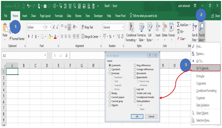
Where do we get this option?

1. Home Tab
2. Find & Select
3. Go to Special

Or

Press short cut key (Ctrl+G or F5, Alt+S)

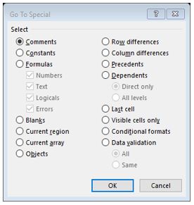
These are the features of “Go to special” Option. Each option has its own speciality. Let’s understand it one by one.

1. Comments– when we want to remove all the comments from the current worksheet.

• Select the database
• Home tab->> Find & select ->> Go to special or Press Ctrl+G, Alt+S
• Click on comments
• Ok

Now we can see all the comments selected automatically. Simply press the delete button and whole comments will be deleted.

2. Constants- when we want to select/highlight the following constants in our excel worksheet-

• Select the database
• Home tab->> Find & select ->> Go to special or Press Ctrl+G, Alt+S

1. Number- Mark this option if we want to highlight the only number
2. Text- Mark this option if we want to highlight only Text
3. Logicals- Mark this option if we wanted to know about those cells which are keeping logical text (TRUE/FALSE)

• Ok

3. Formulas- when we want to select/Highlight the following return values through formula-

• Select the database
• Home tab->> Find & select ->> Go to special or Press Ctrl+G, Alt+S

1. Number- This option selects those formulas which return the number values
2. Text- This option selects those formulas which return the Text values only
3. Logicals- This option selects those formulas which return the logical value only (TRUE/FALSE)
4. Errors- This option selects those formulas which return the Error message.

• OK

4. Blanks- Look at the below mention screenshot-

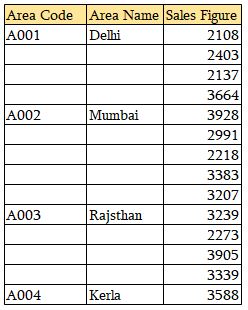
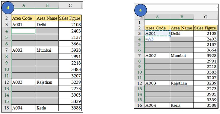
In this database, we want to prepare the area wise sales report, but the area name is missing between the next area name. So, how we can fix this problem? Normal excel user do copy the area code and area name and paste them before the next area code and name. But don’t be the part of the crowd, make our own identity. Instead of doing copy and paste, follow the below mention procedure-

• Select the table (do not select the whole sheet)
• Home Tab->> Find & select->> Go to special
• Choose Blank

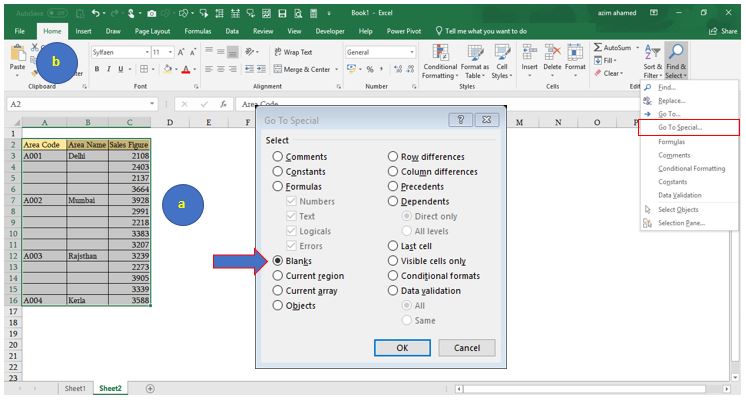
• When we click on Ok, all the blank cell get selected
• Press equal to (=), it will be typed by default in cell A4. choose upper cell A3 with keyboard up arrow key –( )
• Do not press enter, press CTRL-Enter
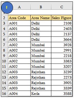
• All the blank cell will be filled with their area code and area name automatically.

                  5. Current Region- This option is useful for the selection of the range where the current mouse located. Put the cursor over the range and choose the current region from Go to Special features. By the way, I always prefer to apply CTRL+* instead of choosing the current region.

                 6. Current Array- It can select the all array function which applied in the current worksheet

                 7. Objects- This option can select all the object like (charts, Shape, image, etc.). when we want to delete all the images, charts and Shape at once. this is the best one. Simply follow the procedure-

1. Select the whole data
2. Find & Select ->> Go to Special
3. Select the object
4. Ok

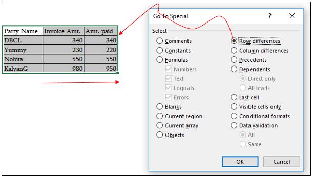
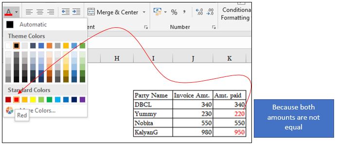
                8. Row Differences- Select the cells that are different from the active cell within the selected row. This is a very useful auditing tool for highlighting inconsistent formula in a row.

                9. Column Differences- It can highlight that is different from the active cell within the selected column. See the demo as explain in row difference.

                10. Precedents – It will select those cells which are responsible for the answer cell

                11. Dependents- It will select those answerable cells which come from the single cell

                12. Last Cell-Select the last used cell within our worksheet

                13. Visible cells Only- This is one of the best features of Go to Special button. when we want to do copy and paste for those cells which are not hidden.

                14. Conditional Formats- This option helps us to find out and select those columns which are keeping conditional formatting. when we click on the option conditional, we get the following option-

1. All- It means it will select conditional formatting from the entire workbook
2. Same- It only selects the same conditional formatting applied in another column

                15. Data Validation – This option helps us to find and select those columns which are keeping data validation.

1. All- It means it will select data validation form the entire workbook
2. Same- It only selects the same data validation applied on another column

So, this is the full information about the “Go to Special” Feature. Do right any question into the comment box. We would love to assist you. Stay tuned and stay connected with Nurture Tech Academy.

Happy Learning 😊