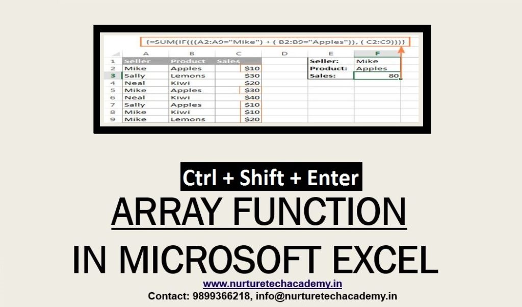
Array function is one of the powerful formulas. Array formula can do multiple tasks and multiple calculations can replace multiple formulae in one cell. And guys, still approximately 80-90% of the people do not know, how to use this formula? And the reason because they scare to learn it.
No doubt, Array function is a little bit confusing to understand and that is why we are here to understand the mystery of this formula. The aim of this blog post, to make you understand the array function in an easy and meaningful way.
Excited! Let’s dive in the ocean of Powerful Excel and learn the most magical “Array Function in Excel”.
Array Formula:
Before we start the array formula in excel, let’s understand, what is the meaning of “Array” is? Array is nothing but the collection of information. by the way, Information can be in the form of “Number” or “Text”.
For example, if we need to fill the employee Name with the array function, the formula looks like this-
{={“Mr.A”,” Mr.B”,” Mr.C”,” Mr.D”,” Mr.E”}
First of all, select the range then type this formula starts with “=” equal sign, once you have completed the formula, Do not press enter, press Ctrl+Shift+Enter
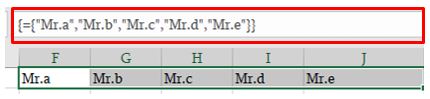
Remember, instead of typing manually in every cell, we just type in one cell and press Ctrl+Shift+Enter. We got the result, and this is what exactly “Array function “does. Not only can an array formula deal with several values simultaneously, but it can also return several values at a time. So, the results returned by an Excel array formula is also an array.
Example:
Just look at this database, if we need to calculate the total amount-
- We will add a column
- We will multiply Price* Quantity in each single cell
- We will apply Sum() formula
- Ok
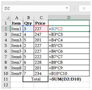
Why did so much task to get the only single cell result? Whereas we have a magnificent “ Array Function” which can do multiple tasks in one time.
There is no need to add another column just put your cursor below of the last price value and apply this formula:
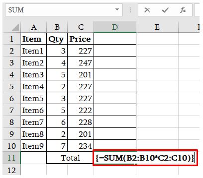
Hope, we understand the power of array function in excel. Suppose, if we have a large amount of data then how much time now we can save from this extremely powerful function.
How can we enter array formula in excel?
There are four things which we must keep in our mind during entering array function-
1- Before starting of formula, we must select the range first. Once we complete the formula, press Ctrl+Shift+Enter. We can check two curly brackets {} will come before and at the end the formula. We can check into the formula bar.
2- Every time when we edit the formula, to circulate the changes in all cell, We must press Ctrl+Shift+Enter, If we forget then it will behave like a simple formula and we will get the result into the first cell only.
3- Remember, we don’t have to manually put curly brackets into the formula, We must press Ctrl+Shift+Enter and the curly brackets will appear automatically.
4- Every time when you open formula, curly brackets will disappear, we have to press Ctrl+Shift+Enter at the end of formula completion.
Example:2
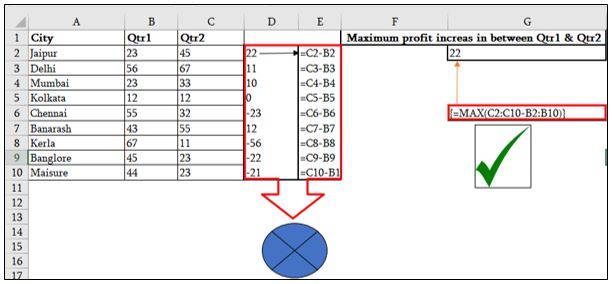
Suppose, if we have two quarter’s data and we want to find out the maximum increase amount in between the quarters. For this, we follow below-mentioned steps-
- We will add a column
- We will subtract the value (Qtr2-Qtr1) by applying this formula in each and every cell
- We will apply the max() formula to get the maximum profit
Instead of doing such a long way process, we can simply do it with the help of Array Function.
Refer to the image below-
Multi-cell array formula:
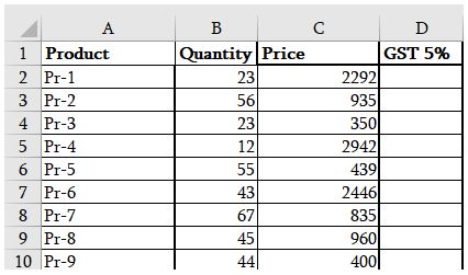
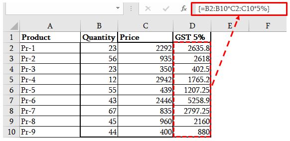
Let’s suppose if we need to calculate GST@5% of each product. How we will do it? We will type a formula Quantity*Price*5% and copied it every cell.
This is an old way, just try this “Array Function” with following given option-
- Select the all blank cell under GST@5% column (D2: D10)
- Press equal to (=)
- Type =(B2:B10*C2:C10*5%)
- Press Ctrl+Shift+Enter
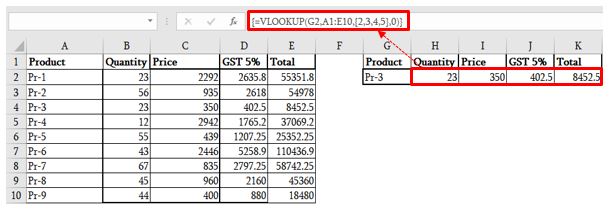
Example 3: Vlookup with array Function
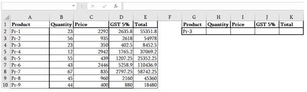
In the above screenshot, Indeed, If we need to find out the product details then we will use VLOOKUP function. But in this case, we have to apply VLOOKUP formula in each cell with a different column number. Unwillingly, we follow this process in our day to day life. Isn’t it.
There is no need to apply VLOOKUP multiple time now on words. Just follow the steps-
- Select the range (H2: K2)
- Type = equal to, it will type in the first cell of selection by default
- Type this formula =VLOOKUP(G2,A1:E10,{2,3,4,5},0)
- Hit Ctrl+Shift+Enter altogether
- See the magic
Note: Inside the Vlookup, column number are showing in between the curly brackets {}
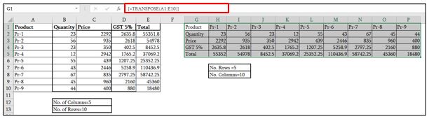
Example 4: Transpose Array
When we need to transpose vertical data in horizontal or Horizontal data into vertical, we follow this procedure-
- Select the data
- Copy
- Choose location somewhere else
- Paste special (Ctrl+Alt+V)
- Click on Transpose
- Ok
However, if we make any changes in old data, will it be automatically updated in transpose data? And the answer is “No”.
This problem can also be resolved with the help of Array Function. Just follow the process-
- Select the number of rows and column just opposite of our old data. For example, refer to the below-mentioned screenshot, In our previous data has no. of columns=5 and no. of Rows= 10, so, we will select 10 columns and 5 rows somewhere else.
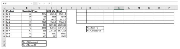
2. Type the formula =TRANSPOSE (A1: E10)
3. Press the Ctrl+Shift+Enter all together
4. Done
Note: If we make any changes in our previous data, changes will update in transpose data automatically. Just try it.
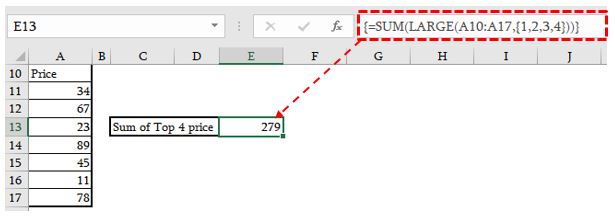
Example 5:
Sum of N number of large numbers in the range:
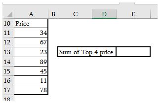
We have a list of the number of prices however, we need to get Total of Top 4 Price value of the product.
We can simply use this formula- =sum(large(A10:A17,{1,2,3,4}) and press Ctrl+Shift+Enter
Similarly, If we need 3 smallest price = sum (Small (A10:A17,{1,2,3}) & Ctrl+Shift+Enter
In a similar fashion, we can calculate the average-
Average of Top 3 price- =average (Large(A10:A17,{1,2,3}) & Ctrl+Shift+Enter
Average of 3 Smallest price- =average(small(A10:A17,{1,2,3}) & Ctrl+Shift+Enter
We hope this blog post helps us to understand the meaning and powerful use of array function. Just try these examples in your practical database, if occur any problem or if you have any queries. Feel free to write it down in the comment box or connect us. Also, guys, you can mention the topic on which you want a complete blog. We will give you the best shot.
Thank you so much to read this article and stay tuned with nurture tech academy.
Happy Learning 😊