Hi All,
When we think of the analysis of data into excel, what comes first in our mind? Yes! The correct answer is the Pivot table. However, we know that the pivot table has its own limitation and we know that, when we want to do the analysis of any data, we need to convert data into a pivot table format, so that we just drag the heading with mouse and drop it on a proper place, to get the actual report.
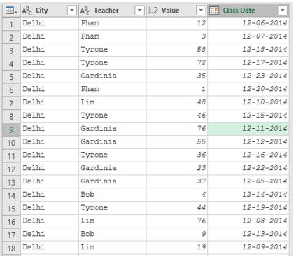
Let’s take an example, just have a look at this screenshot below, this is not a pivot table-
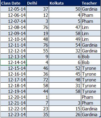
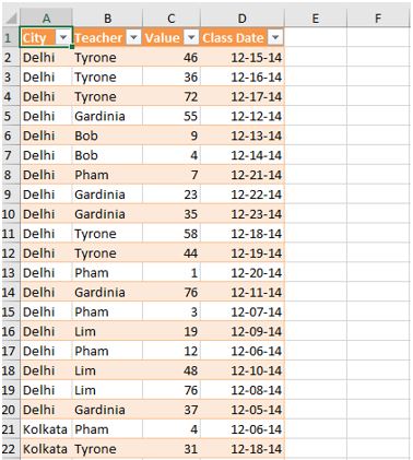
This data we get from a training B school and this report are about, Date wise teacher’s class schedule in the city. However, we want to make this report in this below-mentioned screenshot-
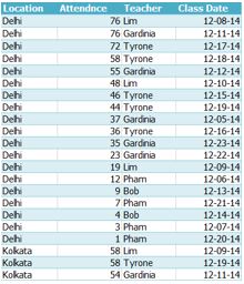
Transpose the headings and its values. Can we do it with the pivot table? Can we do it with simply using option transpose? we don’t think so then should we do it manually copy and paste? manually copy and paste is old style. As we did promise to all that we will make you, champion in Excel. As we always keep our promises.
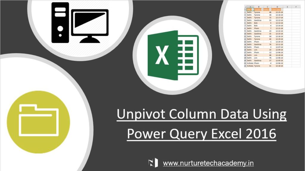
Therefore, we would like to update you a super powerful function in Power Query is called “Unpivot Table”. Microsoft Power query has been introduced by Microsoft earlier. This is the free Add-Ins, we can download it by clicking on this link Download Power Query if we are using Ms-office 2013 but if we are using Ms-Office 2016 then there Is no need to download it. It comes by default with Ms-Office 2016.
So, let’s break the suspense and understand “Unpivot Table” in Power Query.
Unpivot column in Power Query-
Convert the database in Table format first otherwise “Unpivot Table” features would not work. Here are the steps to define how can we convert our data in table format-
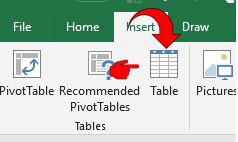
- Select the whole data
- Go to Insert Tab
- Click on Table option
Or
- Select the data
- Press the short cut key (Ctrl+T)
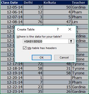
- We can change the range location
- Make sure “My table has headers” option should check mark because new heading will be inserted with the name “Column1”,” Column2” etc if we forget to check this option.
- Ok
when data convert into the table format, follow the below mention steps to complete the task-
- Select the database
- Go to Data Tab
- Click on From Table/Range
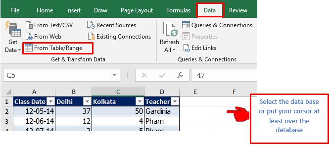
4. When we click on Table/Range, it will take us on a different page. This page is Power Query Editor Page.
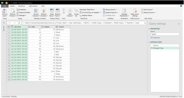
5. Short introduction about Power query Editor-
- File- we can save and close the query editor by clicking on this, feature
- Ribbon Tab- There are four Tab available in Ribbon Tab, like excel
- Formula bar- Power query has, its own M-code natural language
- Query Settings- we can manage the applied steps
Note: We have a separate blog-post for the complete details of these features. We can visit on blog-post column to read the full article
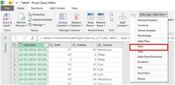
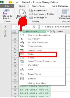
6. Change the date format in “Date” only, it is coming date with time
- Select the class date
- Click on Home Button in Ribbon Tab
- Click on Date Type:
- Select the option “Date”
Or
- Click on icon showing upper left corner of the heading “Class Date”
- Select “Date”
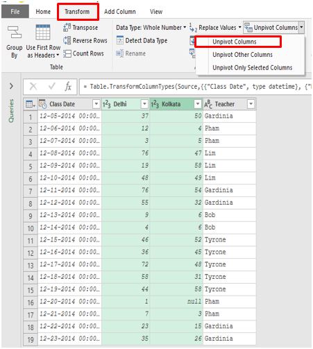
7. Select the both Heading “Delhi” & “Kolkata” both together
8. Go to Transforms in Ribbon Tab
9. Click on Unpivot Columns
10. After a click, both columns merge into one column with the name Attribute
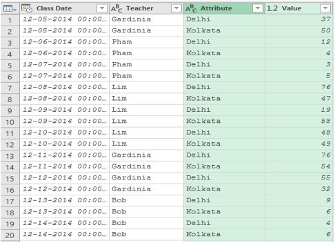
11. Double click on the name “Attribute” and change the name “City”
12. Click on Filter->> Sort the data in Ascending order
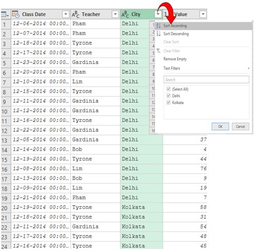
13. Exchange the heading in chronological order
- City
- Teacher
- Value
- Class date
Note: Simply drag it with holding the left key of your mouse and drop it
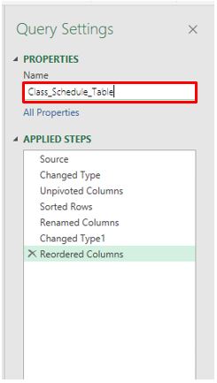
14. Once all done, define a name “Class_Schedule_Table” to this query inside the properties option, which is locating on the right side of the dialogue box
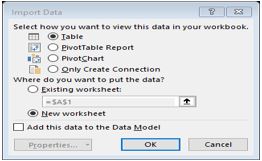
15. Home->> Close & Load
- Close & load- Power Query editor will be closed, and data will import in a new sheet

- Close & Load to- Power query editor will be closed but we will get a new dialogue box in which we can choose the format and location to import the data
16. Data will be imported into the Excel in Table Format
Hope, this blog-post help us to understand the unpivot column in power query. Download the practice file and do the practice. If you have any query or question, feel free to write it down into the comment box or directly contact us. We would be happy to help you.
Thank you so much to read this blog-Post. Stay tuned to nurture tech academy.
Happy Learning 😊