
Hi,
Conditional formatting is the best way to visualize data in a colourway. With conditional formatting, we can do things like highlights data into colours, apply bars, Icons, Flags and formulas.
As an Excel user, we usually highlight data into colours however in the practical scenario we are applying colour manually which is a time-consuming process.
This blog post will help you to apply colours with the help of a drop-down list. In the drop-down list we have text list i.e. Salesman & Types etc. once you select the name, the colour will apply accordingly. Refer the image given below-
isn’t cool!
Today we will learn how we can use Conditional formatting through Data Validation. Let’s dive into the ocean of colours and condition.
Step1: As you can see below, we have a dummy data, Workbook having a Sales report and we want to highlight the report as per my salesman and it’s selling type i.e. Cash or Credit.
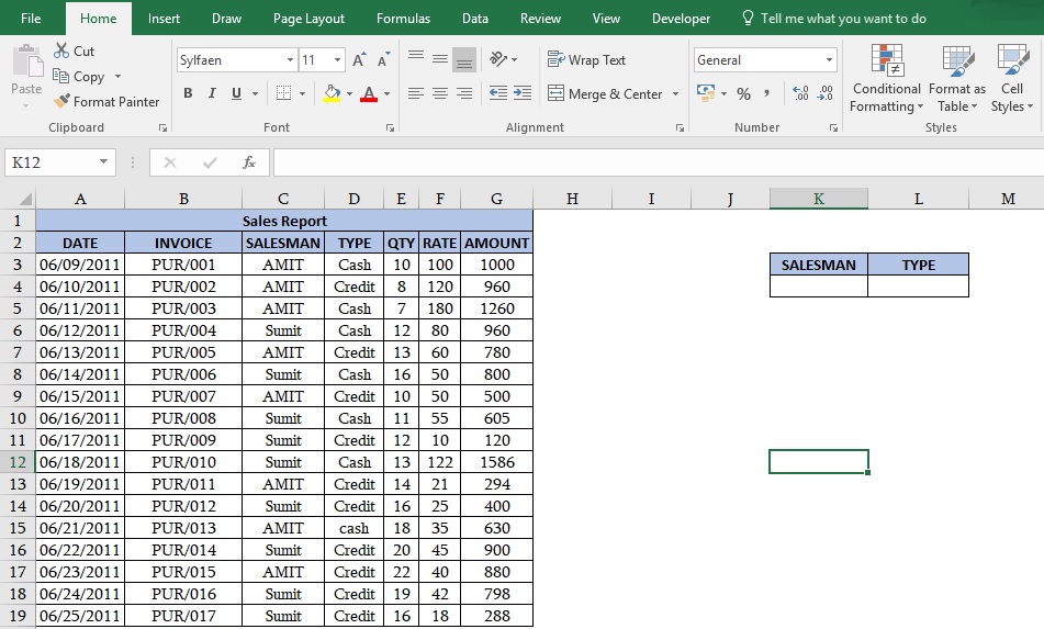
Step2: First, we must create a drop-down list in cell K4 and L4.
How can we create a drop-down list?
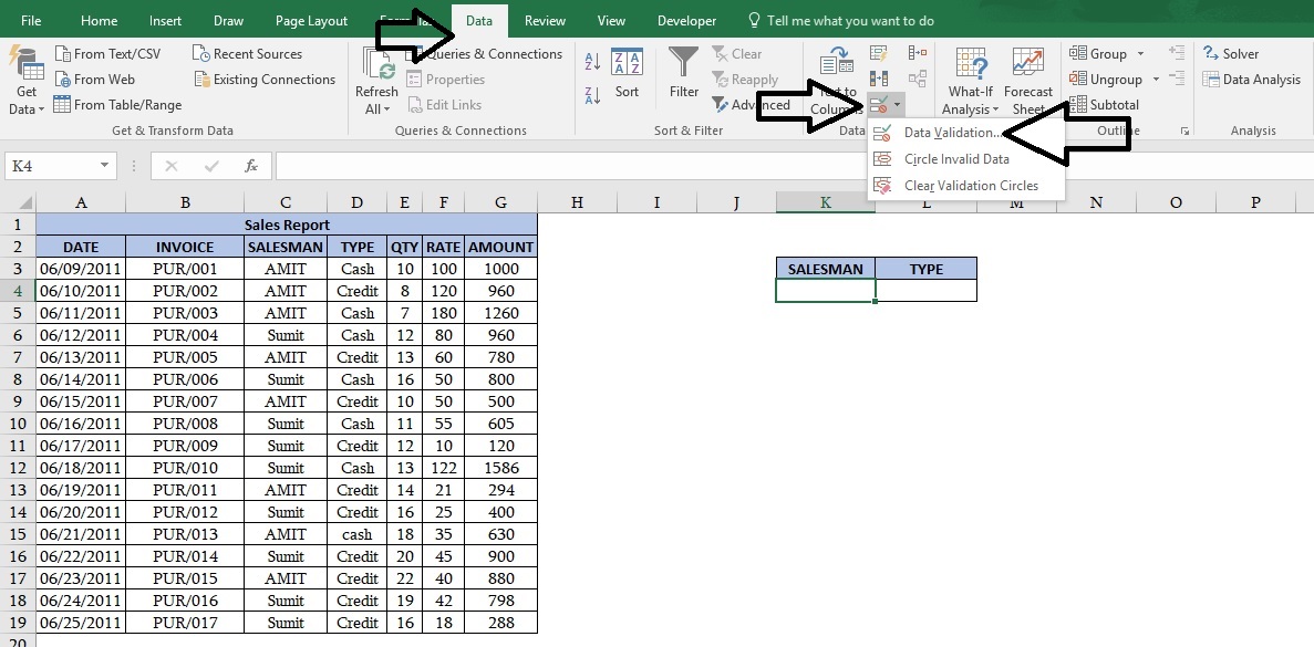
Go to Data tab-> Data validation-> Settings-> Any value-> select List option (Refer image given below)
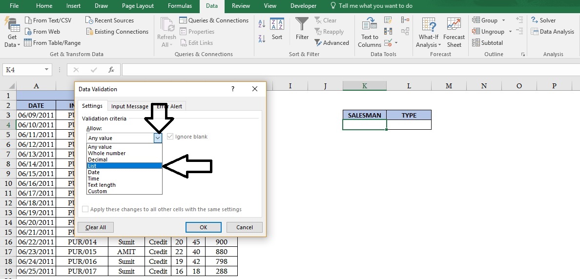
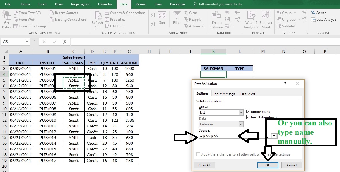
In source box either you can select salesman list form your existing data or you can type it manually E.g. Amit, Sumit.
Note: You can create a separate list anywhere else and select them.
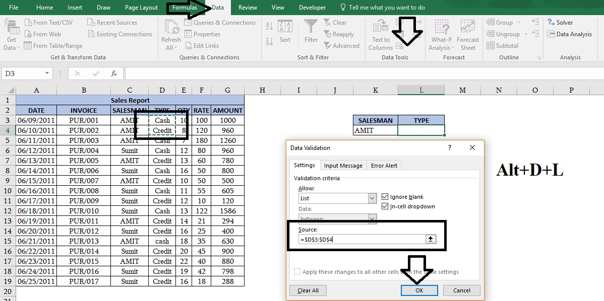
Instead of going manually, we can open data validation through the Keyboard shortcut key “Alt+D+L”.
Follow the step2 and create a drop-down list for the heading “Type”.
Step 3: Drop-Down list done. Select data without heading-> Home -> Conditional Formatting-> New Rule
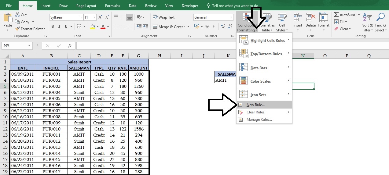
Click on New Rule-> new dialogue box will be open-
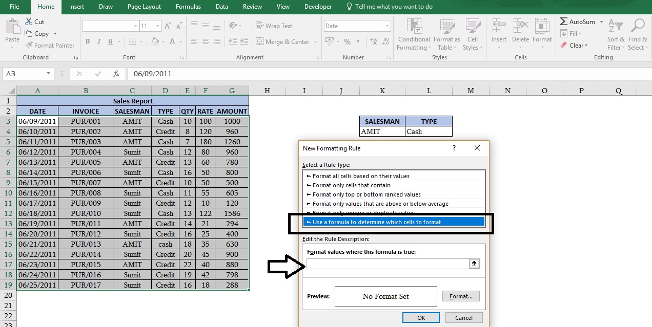
Select option-> “Use a Formula to determine which cell to format”-> Now in this box we will apply a formula as given below-
If(And($C3=$k$4, $D3=$L$4),”True”, “False”)
Using If function-
=If(Logical Test, Value if true, Value if false)
Logical test- With the help of If function we can apply a logic in between two cells or more.
where you would give logical value. In another way, we can say what you want to do.
Value if true- If excel finds any value which is equivalent to your given logics then it will revert you True value as you give in your logical test.
Value if False- If excel could not find the value which is equivalent to your given logics then it will revert you a false as you give in your logical test.
Using If with AND function-
And is the most useful member of the Logical family. When you have more than one condition and all condition are mandatory then we use AND function.
=IF(And(Logical1,Logical2,Logical3,……..)
Mixed cell reference- A mixed cell reference is either absolute column and relative rows or absolute rows or relative columns. When you add $ sign before the column, it means Column will be freeze and row will be a relative reference. For Example- $C3 is absolute for column C and Row 3 is for relative reference or C$3 is absolute for Row 3 and Column C is a relative reference.
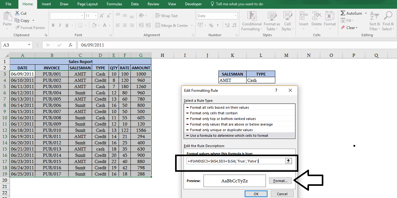
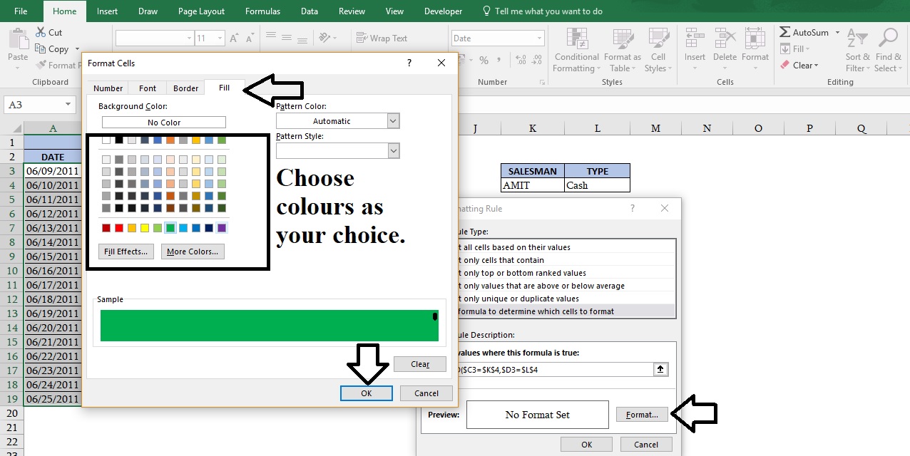
Step4: After apply the formula” If(And($C3=$k$4, $D3=$L$4),”True”, “False” -> Format->Fill->Select any colours->OK
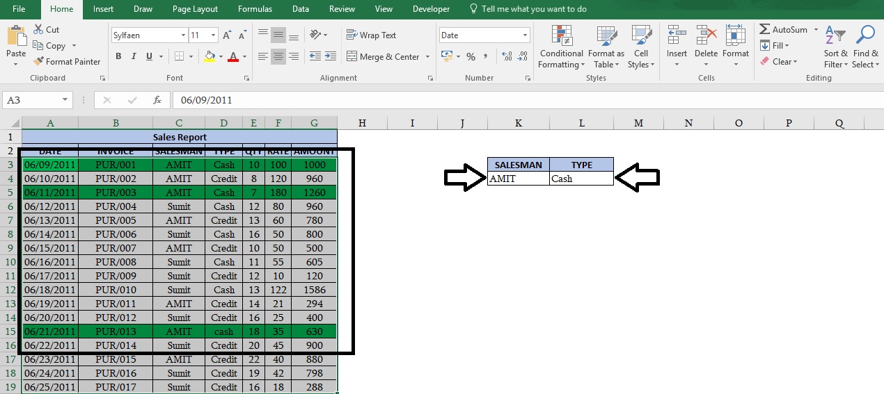
All done! Select salesman and type from drop-down list E.g. Amit and cash and you will see data will be highlighted as per your selection.
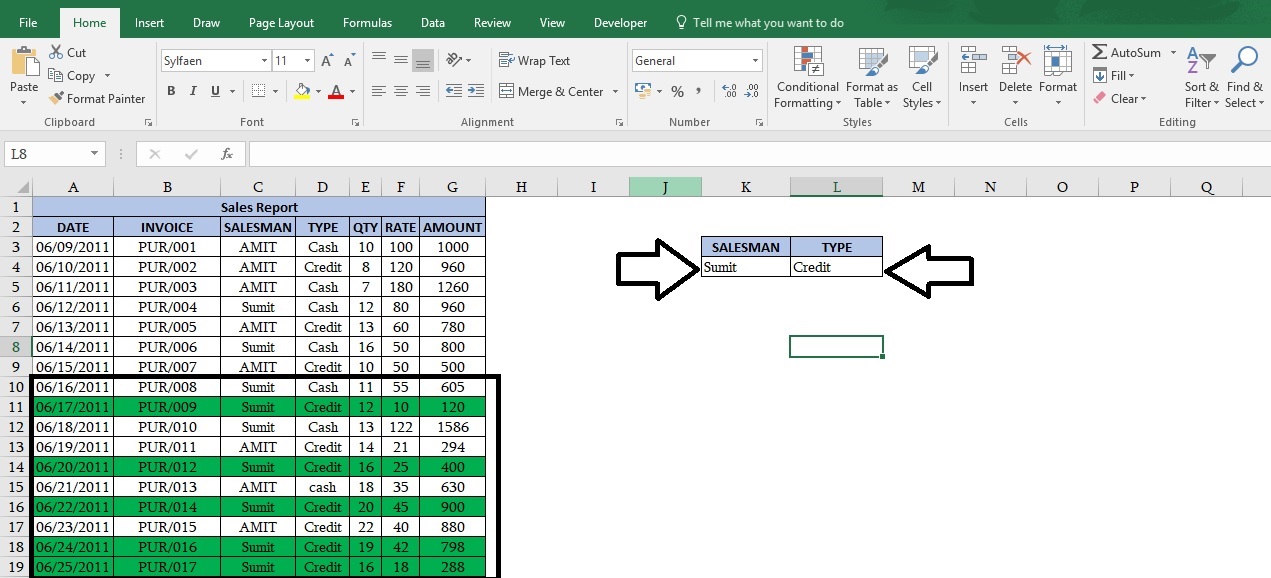
When you will change our salesman and their types, Data will be formatted accordingly.
Enjoy!
you can download the practice file by clicking on this link- Practice File
Happy Learning😊