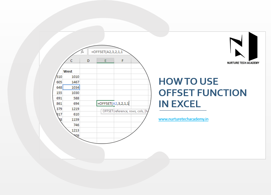
In this article, we would put lights on the most mysterious concern of all time in Excel The Offset Function.
So, what Offset does in Excel? Basically, the OFFSET formula returns a reference to a range that is offset from a starting cell or a range of cells by a specified number of rows and columns.
Excited! Let’s understand this mystery and apply the Offset function in a better way. I’ll explain it in a simple and meaning full way. So, let’s not waste the time, dive into the ocean of Excel.
Excel Offset function- Syntax
The Offset Function return the value of a cell or range that depends on how much row and columns we mentioned.
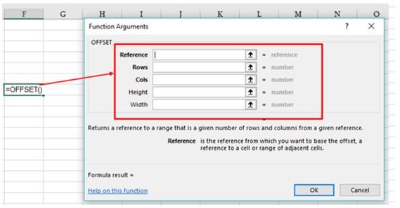
As I have already explained that there are two types of arguments in any formula-
- Mandatory/Required -which shows in Bold letter (see in the above image first three)
- Optional – Non-bold letter (last 2 see in the above image)
These arguments help us to understand what you are supposed to specify in a cell.
Mandatory Arguments-
- Reference- A cell or a range of adjacent cell which you base the value. Basically, we can say this is the first point of any formula.
- Row- This helps to move the rows to up & Down from the starting point. Remember, If the values of the row are positive then formula move down from the reference point if the value is negative then formula goes above from the starting point.
- Cols- This helps us to move the cell, left to right from the starting point.
Optional Arguments: –
- Height- the height, in number of rows, of the returned reference
- Width- the width, in number of columns, of the returned reference
And now, let’s understand this theory through practical examples-
Example: 1
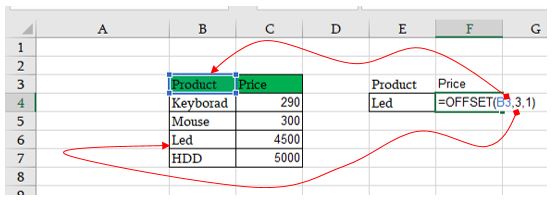
Let’s understand, how it works, As explained in above Offset, start with “Reference (B3)”, start the counting for the row number next from the reference(B3) and that is 3 and start the count column from the cell reference and that is column number is 1.
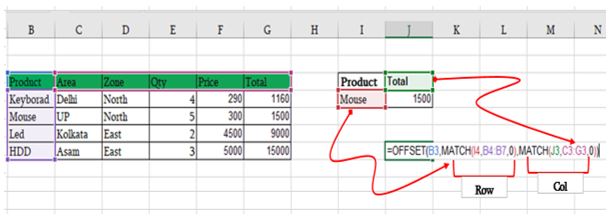
Offset function with match function-
In the above example, if we change the product name, price value will not be updated automatically because in the above example we define row number manually. Isn’t it?
To get rid of this formula we can use “match” function which tells us the exact position of cell address.
Match function does the exact position, which we consider as a number. Look at the example below-
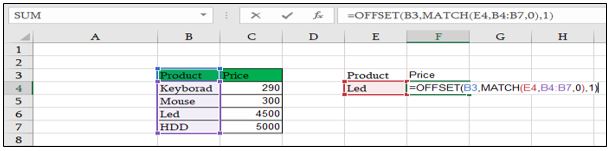
Now we only change the name in the cell (E4) and the price will update automatically.
Note:- similarly, to get the column and row’s value at the same time, we can use the formula as given in below mention image.
Example-2
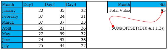
Look at this example, we need to calculate the Total value of 4th row ‘s entire column. –
Sum (Offset(B10,4,1,1,3))
B10- Reference
- 4- Start from the 4th row
- start counting from column 1
- add data from the 1 row only
- add data from the entire column which are 3 (Day1, Day2, Day3)
Note: If we type this formula Sum (Offset(B10,4,1,2,3)), it means it will add 2rows and 3 column’s value.
Why do we use the Offset Function in Excel?
As of now, we understand what Offset Function does, However, one question can disturb you that “why we bother for this formula whereas we can simply use the formula sum and select the range.”
Friend, the Situation is not like that.
Dynamic Range: when we apply sum function on a specific range, we got the result. But we have a worksheet where a new row or column is added every week than in this case dynamic range help us a lot.
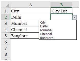
Dynamic List – Excel Offset Function-
Dynamic range features are most useful in different scenarios with the help of COUNTA function. For example, it can help to create a drop-down list.
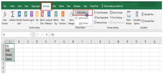
Follow the steps-
- Define Name Range
- Select your list
- 2-Go to formula
- Define name ->> Type Name (Data)
- 4-Ok
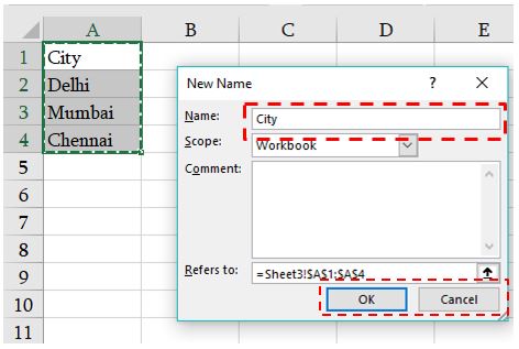
- Define Dynamic Range
- Go to Formula
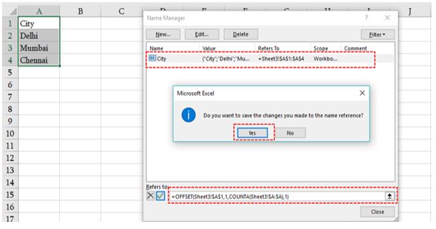
- Name manager
- Select the Name (“City”)-
- Apply this formula inside the box “Refers to” =OFFSET(Sheet3!$A$1,1, COUNTA(Sheet3!$A:$A),1)
- Once the formula has done ->> click on “City”
- Click on “Yes”->> Close the window
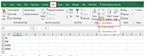
- Create a Drop-Down list
- Select Cell B2->> Go to Data Tab
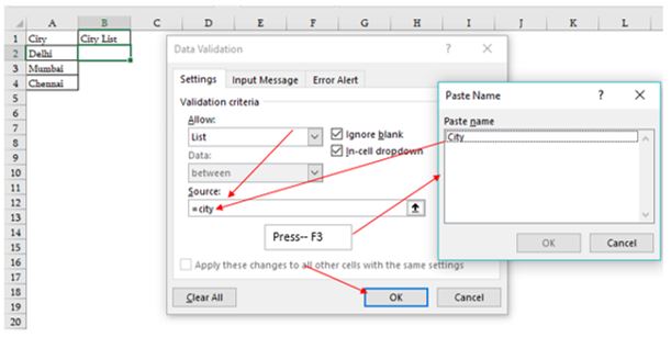
- Data Validation
- List-> Click on Source->> Press “F3”->> Select “City”
- Ok
Do we remember the question asked at the beginning of this tutorial- “What is OFFSET in Excel? We hope now we know the answer 😊
If you guys have any query or question, feel free to ask in the comment box or you can directly contact us. We would love to solve your query.
Thank you so much for reading! 😊