How to use Pivot Table in Microsoft Excel

Hi Guys,

When we are dealing with large data set in excel, Pivot table comes in the right way to help us to create an interactive summary from different records. Apart from these things, the pivot table automatically do short the data and apply the filter button as well. Also, it can Create a tabulation report, calculate the total sales & average.

Another benefit of using a pivot table, we can create a stunning summary report by just dragging and dropping option the source table column and this feature gives it name Pivot Table.

Being as an Excel Trainer and user, I can say the pivot table is the backbone of Excel. So, let’s jump into the ocean of pivot table and learn this extraordinary feature of Ms-Excel.

Pivot Table-

A PivotTable is a powerful tool to calculate, summarize, and analyse data that lets you see comparisons, patterns, and trends in your data.

Source Microsoft Office

Let’s understand, what Pivot Table can do for us-

1. It does Summarise data by categories and Subcategories
2. It can present our big database in a friendly way
3. It can do data sort, Apply Filter, conditional formatting which helps us to identify our most important information
4. Simply drag and drop and database can switch between rows and columns
5. Expand and collapse button applied to our database which drills down on the behind data
6. Aggregate and subtotals numeric data in the spreadsheet
7. it does Multiple calculations without using any formula, all the formulas are by default exist
8. it does data refresh
9. Pivot Chart which makes pivot report along with the chart

For Example –

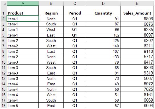
In the above screenshot, we have a Region_wise_Sales workbook having thousands of data. If we want to calculate Region and product wise sales Report. One possible way to calculate it by using formula SUMIF & SUMIFS or we do apply filter option to get data. Somehow, we do prepare our report but we all know, it takes a lot of time. If we do prepare this report with the help of pivot table, just a few mouse clicks and our summary report get to be ready in an elegant way.

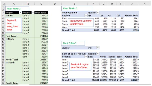
The above screenshot demonstrates how easily we can create these possible layouts with the help of the Pivot Table. Further, we will discuss in below mention steps that how we can create this through the pivot table in the office version 2016,2013,2010 & 2007.

How to convert data into the Pivot Table-

Before converting our data into the pivot table, Organize our data row and column wise. Convert your data into Table Format because, after table format, data behave dynamically. In this context, A dynamic range means it will automatically shrink and expand the data as you add or remove the database. So, we won’t have to worry about that pivot table is missing the new data updated in Table 😊

Make sure the database does not contain any blank rows or columns and no subtotals. Define a name to our database with following steps-

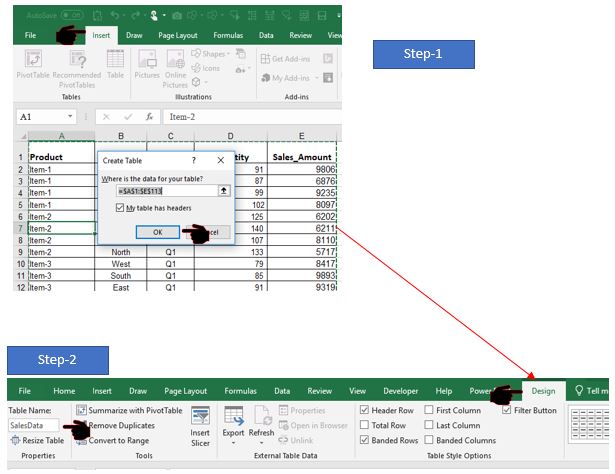
Next step to convert the database into the Pivot Table with the following steps-

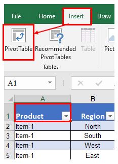
1. Select any cell in the source table
2. Go to Insert Tab
3. Pivot Table
4. Or Press short cut key ALT+N+V

Note: There is no need to select and hold the data, put the cursor over the table.

This will open the window “Create Pivot Table”.

Select a Table or range- Here, the selection of table range highlighted inside the Table/Range box. In our example, it’s showing Sales Data because we have taken the Table range Sales Data.

New Worksheet- It means, the Pivot table will be created on a new sheet.

Existing Worksheet– It means, not only on this sheet but also, we can create the pivot table in all existing sheet. Click into the box Location and define the location where we want to create the pivot table.

Note: As this pivot table is for beginner, later we will discuss the rest two option which is related with Data Model.

Clicking the OK button, it creates a blank pivot table into the define location. For example, for this database, we are selecting New worksheet. It means a blank pivot table will be created a new worksheet. Which is quite look like this-

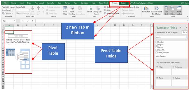
Let’s discuss the Pivot Table Fields option-

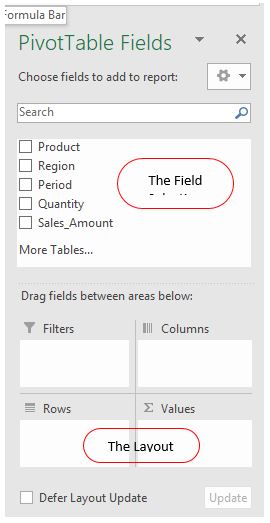
The area where we work with the fields of our summary reports is called the Pivot Table Field List. It is in the right-hand part of the sheet and divided into two part-

1. The Field Selection- The Field selection contains the name of the field which we can use to create a pivot table report. The field name corresponds to name of our columns from the source table
2. The Layout Selection- This option contains Report Filters, Columns, Rows, and Values. Here we can arrange and re-arrange the fields of our table

The changes which we made into the pivot table field list, immediately it will reflect into the Pivot table.

How to add a file to Pivot Table in Excel-

To add a filed into the layout, select the checkbox to appear into the field selection option. When we click, it will reflect into the layout box with following rules & regulation-

1. A filed which consisting only Text (Non-Numeric values) will be reflecting into the Row layout
2. A filed which consisting only Numbers will be reflecting into the layout of the values
3. Online Analytical Processing (OLAP) date and time hierarchies are added to columns value by default

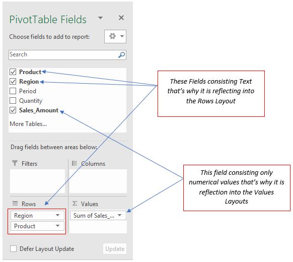
When we put down our field into their specific place. The report will look like this. (See Below)

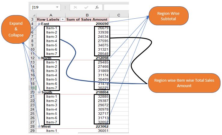
If we put light on the above pivot summary report screenshot, It shows Subtotal of each region along with item and its value. We can expand and collapse the report by click on this icon. 

Let’s arrange the pivot table fields-

We can arrange the Table fields in Layout in three ways-

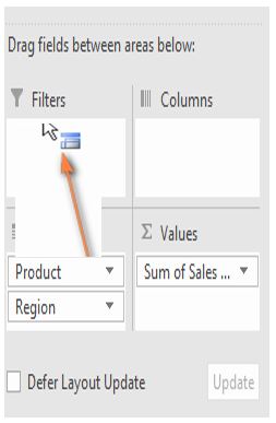
1. Drag-Drop- The first and most useful way to fit the heading inside the layout box. Simply drag the heading through mouse with the holding of left key and drop into the field where we want. This will remove the current area and place it in a new area.

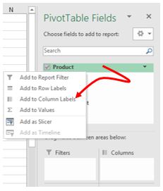
2. Right click on the area and choose the location where we want to add it.

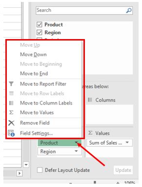
3. Click on the field drop down, it will keep the same option where we can select the destination

Values option in Pivot Table-

By default, when we drag any numerical values inside the Value layout section. It comes with auto SUM by default. When we drag any non-numeric value or any Boolean number into the value field layout. it counts it. But of course, we can choose different function with the following option-

1. Click on the value field
2. Value field option
3. Summarise values by

Or

1. Right click on the number
2. Summarise values by
3. Choose the option

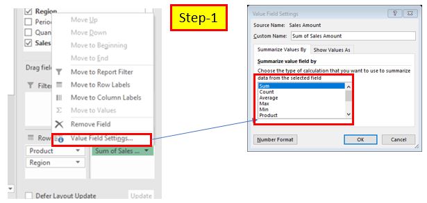
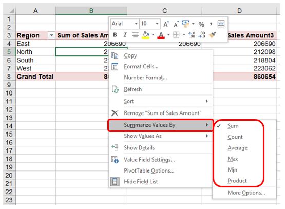
• Simply select any one and values become change. For example, IF we want to prepare a report based on Region wise Total Sales, Total Average, Total Count, Max, and Minimum, etc. Follow the steps-
• Drag region field into the rows
• Drag sales heading 5 times into the values

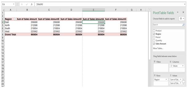
• So, As we can see that the first sales amount is by default Total Sales Amount. So, we will click on the second one
• Summarize values by
• Select average

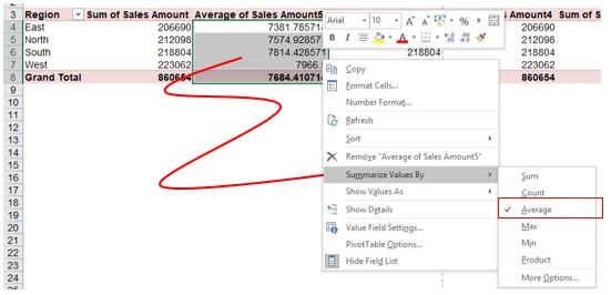
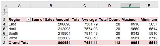
As demonstrated above into the screenshot, when we choose the values converts into the average. Similarly, we follow the same procedure and will choose the option like count, Max & Min each time. In the end, we have 5 reports in a single frame. Refer the below mention screenshot-

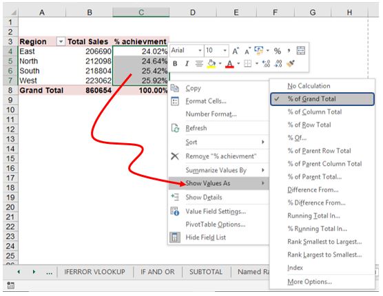
Calculate Percentage in Pivot Table-

when we talk about the percentage of achievement in every zone. This is another feature of Microsoft Pivot table that we can calculate such a thing without using any formula or function. Let’s do it-

1. Drag region into the Row layout
2. Drag sales amount 2 times into the values layout box
3. Right click on the second sales amount
4. Choose the option “Show values as”
5. Click on % of Grand Total
6. Ok

Refresh the Data-

Although we know that our pivot table data has related to some other data source. And it hard to accept that whenever we update some data into our database, Pivot table does not update the table automatically. We do it manually or we can set the pivot table that whenever this workbook will be open, Pivot table get a refresh.

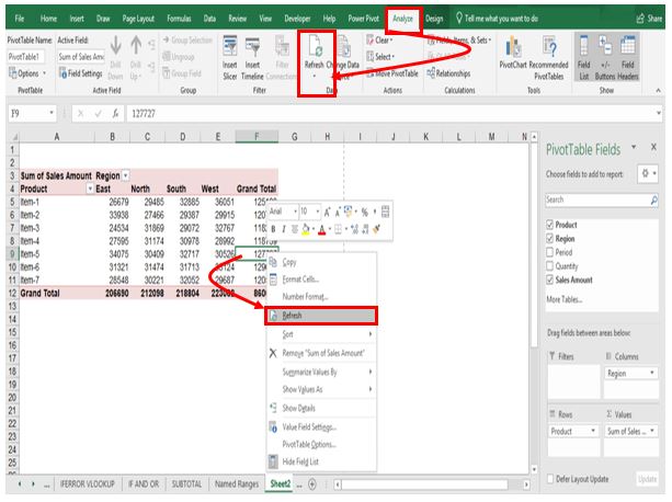
How to refresh data manually-

1. Right click on the pivot table
2. Click on refresh

Or

1. Go to Analyze tab (Pivot table Tool)
2. Click on Refresh or press short cut key Alt+F5

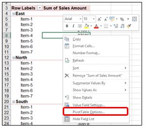
Data refresh when workbook open-

we have just understood above that data refresh is a manual process however we can set our data in such a manner whenever we open our workbook, data refresh automatically. To do this setting, do follow the given below steps-

1. Right click on the pivot table
2. Pivot table options
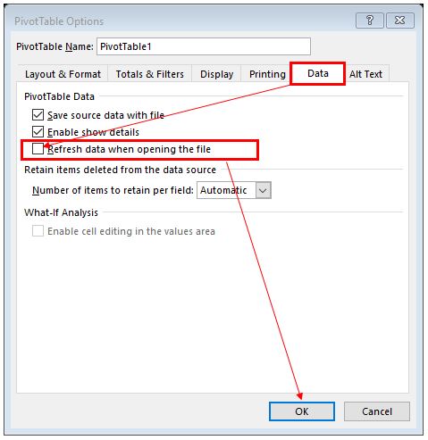
3. Data Tab
4. Checkmark on the option “Refresh data when opening file”
5. Ok

We hope that you like this blog-post. Do apply to your database and tell us how this blog-post helps you. You can write it down into the comment box.

Stay tuned with Nurture Tech Academy.

Happy Learning 😊